Sumif Between Two Dates Things To Know Before You Get This
You use the SUMIF feature to sum the values in an array that meet standards that you specify. For instance, suppose that in a column that has numbers, you desire to sum only the values that are larger than 5. You can utilize the adhering to formula: =SUMIF(B 2: B 25,"> 5") This video clip becomes part of a training program called Include numbers in Excel.
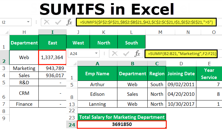
For instance, the formula =SUMIF(B 2: B 5, "John", C 2: C 5) amounts only the worths in the variety C 2: C 5, where the matching cells in the range B 2: B 5 equivalent "John." To sum cells based upon numerous requirements, see SUMIFS function. SUMIF(range, criteria, [sum_range] The SUMIF feature phrase structure has the adhering to debates: array Needed.
Cells in each variety must be numbers or names, ranges, or recommendations which contain numbers. Space and text values are neglected. The selected variety may have dates in basic Excel style (instances listed below). standards Called for. The standards in the type of a number, expression, a cell referral, text, or a feature that defines which cells will certainly be added.
Essential: Any message requirements or any kind of standards that includes sensible or mathematical symbols must be enclosed in dual quote marks ("). If the standards is numeric, dual quote marks are not needed. sum_range Optional. The actual cells to add, if you want to include cells other than those defined in the range argument.
More About Sumif Excel
You can make use of the wildcard personalities-- the enigma (?) and asterisk (*)-- as the standards disagreement. An enigma matches any solitary personality; an asterisk matches any type of sequence of personalities. If you wish to locate a real enigma or asterisk, kind a tilde (~) preceding the personality. The SUMIF function returns incorrect outcomes when you utilize it to match strings longer than 255 characters or to the string #VALUE!.
The real cells that are added are identified by utilizing the upper leftmost cell in the sum_range debate as the beginning cell, and afterwards consisting of cells that match in size and shape to the array disagreement. For instance: If variety is And sum_range is After that the actual cells are A 1: A 5 B 1: B 5 B 1: B 5 A 1: A 5 B 1: B 3 B 1: B 5 A 1: B 4 C 1:D 4 C 1:D 4 A 1: B 4 C 1: C 2 C 1:D 4 However, when the range and also sum_range debates in the SUMIF feature do not have the same variety of cells, worksheet recalculation may take longer than expected.
For formulas to reveal results, select them, press F 2, and after that press Get in. If you need to, you can readjust the column widths to see all the information. Residential Or Commercial Property Worth Compensation Data $100,000 $7,000 $250,000 $200,000 $14,000 $300,000 $21,000 $400,000 $28,000 Formula Description Outcome =SUMIF(A 2: A 5,"> 160000", B 2: B 5) Amount of the commissions for building values over $160,000.
$900,000 =SUMIF(A 2: A 5,300000, B 2: B 5) Amount of the compensations for residential or commercial property worths equal to $300,000. $21,000 =SUMIF(A 2: A 5,">" & C 2, B 2: B 5) Amount of the compensations for residential or commercial property worths above the worth in C 2. $49,000 Example 2 Replicate the example information in the following table, as well as paste it in cell A 1 of a new Excel worksheet.
5 Easy Facts About Sumif Date Range Described
If you require to, you can readjust the column widths to see all the information. Group Food Sales Vegetables Tomatoes $2,300 Veggies Celery $5,500 Fruits Oranges $800 Butter $400 Vegetables Carrots $4,200 Fruits Apples $1,200 Solution Summary Result =SUMIF(A 2: A 7,"Fruits", C 2: C 7) Amount of the sales of all foods in the "Fruits" category.
$12,000 =SUMIF(B 2: B 7,"* es", C 2: C 7) Amount of the sales of all foods that finish in "es" (Tomatoes, Oranges, and also Apples). $4,300 =SUMIF(A 2: A 7,"", C 2: C 7) Amount of the sales of all foods that do not have a classification specified. $400 Top of Page You can constantly ask an expert in the Excel Individual Voice.
To sum if cells contain details message, you can utilize the SUMIF function with a wildcard. In the instance revealed, cell G 6 includes this formula: =SUMIF(C 5: C 11,"* t-shirt *", D 5:D 11) This formula amounts the amounts in ... To subtotal information by group or label, directly in a table, you can utilize a formula based on the SUMIF feature.
To sum if above, you can utilize the SUMIF feature. In the example shown, cell H 6 contains this formula: =SUMIF(amount,"> 1000") where "quantity" is a called variety for cells D 5:D 11. This formula amounts ... To allow a dropdown with an "all" option you can use data validation for the dropdown list, and also a formula based on IF, SUM, and SUMIF features to determine a conditional sum.
All About Sumif Vlookup
To sum if cells end with particular message, you can utilize the SUMIF feature. In the instance revealed, cell G 6 has this formula: =SUMIF(thing,"* hat", quantity) This formula sums cells in the called range amount (D 5: ... If you require to subtotal numbers by shade, you can easily do so with the SUMIF feature.
To sum if cells include certain text in another cell, you can utilize the SUMIF feature with a wildcard and also concatenation. In the example revealed, cell G 6 contains this formula: =SUMIF(C 5: C 11,"*"& F 6 & ... To sum numbers based on other cells being equivalent to either one worth or one more (either x or y), you can use the SUMIF feature.
The ... To conditionally sum the same varieties that exist in separate worksheets, all in one formula, you can do so with the SUMIF feature + INDIRECT, covered in SUMPRODUCT. In the instance, the formula looks like this: =... If you need to sum worths when cells are equal to among several things, you can use a formula based on the SUMIF and also SUMPRODUCT features.
sumif excel practice sumif excel with vlookup excel sumif subtract